Service for Solving Linear Programming Problemsand other interesting typical problems |
Русский | |
Example №7. Solving a Linear Programming Problem Using a Graphical Method.
Function Increases Unlimitedly
F = x1 + x2
subject to the constraints:
| 3 x1 | + | 2 x2 | ≥ | 6 | ||
| - x1 | + | x2 | ≤ | 1 | ||
| x1 | - | 2 x2 | ≤ | 1 |
x1 ≥ 0 x2 ≥ 0
Points whose coordinates satisfy all the inequalities of the constraint system are called a region of feasible solutions.
It is necessary to solve each inequality of the constraint system to find the region of feasible solutions to this problem. (see step 1 - step 3)
The last two steps are necessary to get the answer.
(see step 4 - step 5)
This is a standard solution plan. If the region of feasible solutions is a point or an empty set then the solution will be shorter.
See the plan for solving this problem in pictures
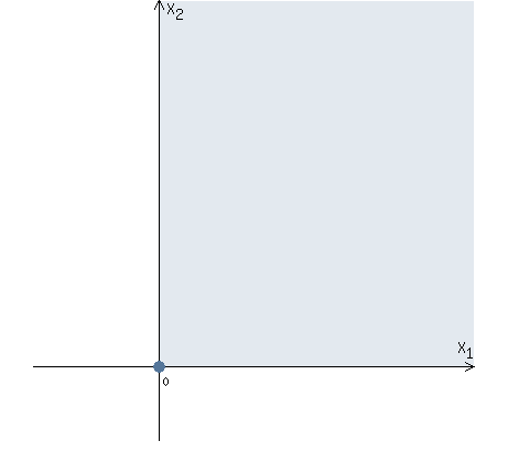
By the condition of the problem: x1 ≥ 0 x2 ≥ 0.
Now we have the region of feasible solutions shown in the picture.
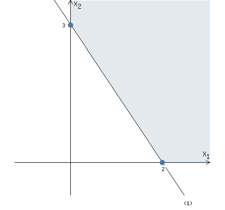
Let's solve 1 inequality of the system of constraints.
3 x1 + 2 x2 ≥ 6
We need to plot a straight line: 3 x1 + 2 x2 = 6
Let x1 =0 => 2 x2 = 6 => x2 = 3
Let x2 =0 => 3 x1 = 6 => x1 = 2
Two points were found: (0, 3) and (2 ,0)
Now we can plot the straight line (1) through the found two points.
Let's go back to the inequality.
3 x1 + 2 x2 ≥ 6
We need to transform the inequality so that only x2 is on the left side.
2 x2 ≥ - 3 x1 + 6
x2 ≥ - 3/2 x1 + 3
The inequality sign is ≥
Therefore, we must consider points above the straight line (1).
Let's combine this result with the previous picture.
Now we have the region of feasible solutions shown in the picture.
Let's solve 2 inequality of the system of constraints.
- x1 + x2 ≤ 1
We need to plot a straight line: - x1 + x2 = 1
Let x1 =0 => x2 = 1
Let x2 =0 => - x1 = 1 => x1 = -1
Two points were found: (0, 1) and (-1 ,0)
Now we can plot the straight line (2) through the found two points.
Let's go back to the inequality.
- x1 + x2 ≤ 1
We need to transform the inequality so that only x2 is on the left side.
x2 ≤ x1 + 1
The inequality sign is ≤
Therefore, we must consider points below the straight line (2).
Let's combine this result with the previous picture.
Now we have the region of feasible solutions shown in the picture.

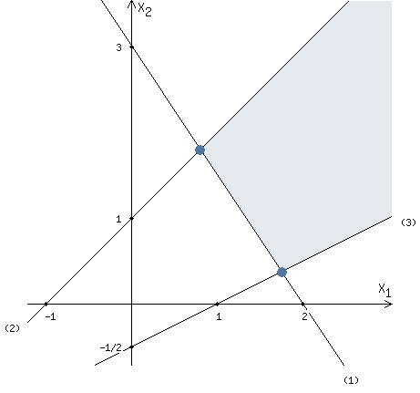
Let's solve 3 inequality of the system of constraints.
x1 - 2 x2 ≤ 1
We need to plot a straight line: x1 - 2 x2 = 1
Let x1 =0 => - 2 x2 = 1 => x2 = -1/2
Let x2 =0 => x1 = 1
Two points were found: (0, -1/2) and (1 ,0)
Now we can plot the straight line (3) through the found two points.
Let's go back to the inequality.
x1 - 2 x2 ≤ 1
We need to transform the inequality so that only x2 is on the left side.
- 2 x2 ≤ - x1 + 1
x2 ≥ 1/2 x1 - 1/2
The inequality sign is ≥
Therefore, we must consider points above the straight line (3).
Let's combine this result with the previous picture.
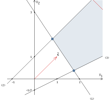
Now we have the region of feasible solutions shown in the picture.
We need to plot the vector C = (1, 1), whose coordinates are the coefficients of the function F.
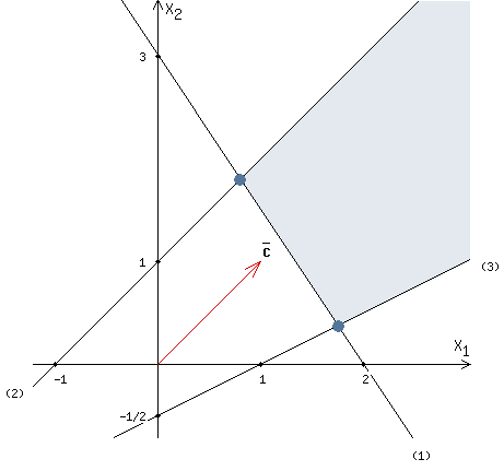
We will move a "red" straight line perpendicular to vector C from the lower left corner to the upper right corner.
The "red" straight line is called the level line. At each point of the level line, the value of the function F is a constant value.
The function F has a minimum value at the point where the "red" straight line crosses the region of feasible solutions for the first time.
The function F has a maximum value at the point where the "red" straight line crosses the region of feasible solutions for the last time.
It is impossible to find the point where the "red" line crosses the region of feasible solutions for the last time, i.s. the function increases indefinitely (see picture).
)
)
)
)
)
)
Fmax = + ∞
© 2010-2024
If you have any comments, please write to matematika1974@yandex.ru