Service for Solving Linear Programming Problemsand other interesting typical problems |
Русский | |
Example №9. Solving a Linear Programming Problem Using a Graphical Method.
Region of Feasible Solutions is a Point
F = x1 + x2
subject to the constraints:
| x1 | + | x2 | ≥ | 1 | ||
| x1 | - | x2 | ≥ | 1 | ||
| x1 | ≤ | 1 | ||||
| 2 x1 | + | x2 | ≥ | 1 | ||
| x1 | + | 2 x2 | ≤ | 7 |
x1 ≥ 0 x2 ≥ 0
Points whose coordinates satisfy all the inequalities of the constraint system are called a region of feasible solutions.
It is necessary to solve each inequality of the constraint system to find the region of feasible solutions to this problem. (see step 1 - step 5)
The last two steps are necessary to get the answer.
(see step 6 - step 7)
This is a standard solution plan. If the region of feasible solutions is a point or an empty set then the solution will be shorter.
See the plan for solving this problem in pictures
By the condition of the problem: x1 ≥ 0 x2 ≥ 0.
Now we have the region of feasible solutions shown in the picture.

Let's solve 1 inequality of the system of constraints.
x1 + x2 ≥ 1
We need to plot a straight line: x1 + x2 = 1
Let x1 =0 => x2 = 1
Let x2 =0 => x1 = 1
Two points were found: (0, 1) and (1 ,0)
Now we can plot the straight line (1) through the found two points.
Let's go back to the inequality.
x1 + x2 ≥ 1
We need to transform the inequality so that only x2 is on the left side.
x2 ≥ - x1 + 1
The inequality sign is ≥
Therefore, we must consider points above the straight line (1).
Let's combine this result with the previous picture.
Now we have the region of feasible solutions shown in the picture.

Let's solve 2 inequality of the system of constraints.
x1 - x2 ≥ 1
We need to plot a straight line: x1 - x2 = 1
Let x1 =0 => - x2 = 1 => x2 = -1
Let x2 =0 => x1 = 1
Two points were found: (0, -1) and (1 ,0)
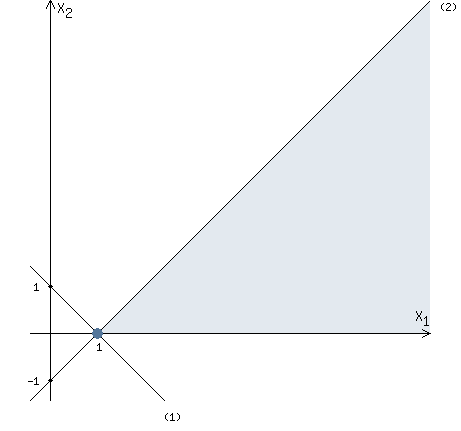
Now we can plot the straight line (2) through the found two points.
Let's go back to the inequality.
x1 - x2 ≥ 1
We need to transform the inequality so that only x2 is on the left side.
- x2 ≥ - x1 + 1
x2 ≤ x1 - 1
The inequality sign is ≤
Therefore, we must consider points below the straight line (2).
Let's combine this result with the previous picture.
Now we have the region of feasible solutions shown in the picture.
Let's solve 3 inequality of the system of constraints.
x1 ≤ 1
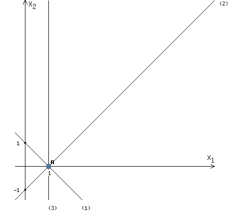
We need to plot a straight line: x1 = 1
Now we can plot the straight line (3) through point (1,0) parallel to the OX2 axis
The inequality sign is ≤
Therefore, we must consider points to the left of the straight line (3).
Let's combine this result with the previous picture.
Now the region of feasible solutions is a point A (see picture).
The coordinates of point A (1,0) are known. (see step 1)
)
)
)
)
We need to check whether the coordinates of point A (1,0) satisfy 4 inequality of the constraint system?
2 * 1 + 1 * 0 ≥ 1
2 ≥ 1
Yes, that's right.
We need to check whether the coordinates of point A (1,0) satisfy 5 inequality of the constraint system?
1 * 1 + 2 * 0 ≤ 7
1 ≤ 7
Yes, that's right.
Let's calculate the value of the function F at point A (1, 0).
F (A) = 1 * 1 + 1 * 0 = 1
x1 = 1
x2 = 0
Fmax = 1
© 2010-2024
If you have any comments, please write to matematika1974@yandex.ru